Introduction
In this blog, we will code and understand the following:
- (1) a linear, single neuron network (no hidden layer),
- (2) the forward propagation function of a deep (non-linear) neuron network with 2 hidden layers,
- (3) loss function (example considered here is cross entropy)
- (4) the workings of Gradient Descent,
- (5) how to train the model, and finally,
- (6) apply all the learnings in building a two-class NN classifier in both Keras and PyTorch
1. Single Neuron
- A linear unit with 1 input

- A liniear unit with 3 inputs > y = w0x0 + w1x1 + w2x2 + b

- In Keras, the input_shape is a list >
model = keras.Sequential([layers.Dense(units=1, input_shape=[3]])> whereunitrepresents the number of neurons in theDenselayer >input_shapedetermines the size of input - where for
- tabular data: >
input_shape = [num_columns] - image_data: >
input_shape = [height, width, channels]
- tabular data: >
- In PyTorch, the same model is defined as follows:
import torch
import torch.nn as nn

class Model(nn.Module):
    def __init__(self):
        super(Model, self).__init__()
        self.fc = nn.Linear(3, 1)

    def forward(self, x):
        x = self.fc(x)
        return x

model = Model()- In PyTorch, the model architecture is explicitly given by subclassing nn.Module and implementing the
__init__andforwardmethods
2. Deep Neural Network
- A dense layer consists of multiple neurons

- Empirical fact: Two dense layers with no activation function is not better than one dense layer
- Why Activation functions?

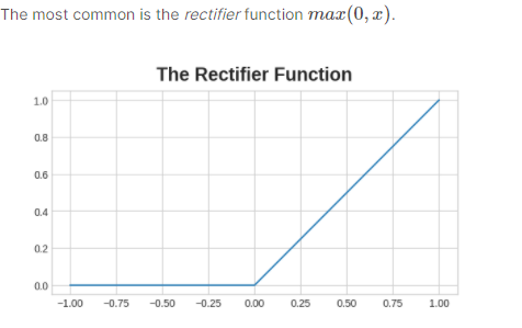
- Rectifier function “rectifies” the negative values to zero. ReLu puts a “bend” in the data and it is better than simple linear regression lines
- A single neuron with ReLu

- A Stack of Dense Layers with ReLu for non-linearity. An example of a Fully-Connected NN:

- the final layer is linear for a regression problem; can have softmax for a classification problem
Keras Version:
from tensorflow import keras
from tensorflow.keras import layers

# defining a model
model = keras.Sequential([
    # the hidden ReLu layers
    layers.Dense(units=4, activation='relu', input_shape=[2]),
    layers.Dense(units=3, activation='relu'),
    layers.Dense(unit=1),
])- The above multilayer NN code in PyTorch can be written as:
import torch
import torch.nn as nn

class Model(nn.Module):
    def __init__(self):
        super(Model, self).__init__()
        self.fc1 = nn.Linear(2, 4)
        self.relu1 = nn.ReLU()
        self.fc2 = nn.Linear(4, 3)
        self.relu2 = nn.ReLU()
        self.fc3 = nn.Linear(3, 1)

    def forward(self, x):
        x = self.fc1(x)
        x = self.relu1(x)
        x = self.fc2(x)
        x = self.relu2(x)
        x = self.fc3(x)
        return x

model = Model()
3. Loss Function
- Accuracy cannot be used as loss function in NN because as ratio (
num_correct / total predictions) changes in “jumps”. We need a loss function that changes smoothly. Cross Entropy= - 1/N ∑ (i=1 to N) {(y_actual(i) * log(y_predicted(i)) + (1-y_actual(i)) * log(1-y_predicted(i)) }- CE is measure to compute distance between probabilities.
- If y_predicted(i) is farther from y_actual(i), CE(i) will be closer to 1. Vice versa, if y_predicted(i) is closer to y_actual(i), then CE(i) will be close to 0

4. Gradient Descent
- Gradient Descent is an optimization algorithm that tells the NN
- how to change its weight so that
- the loss curve shows a descending trend

Definition of terms:
Gradient: Tells us in what direction the NN needs to adjust its weights. It is computed as a partial derivative of a multivariablecost funccost_func: Simplest one: Mean_absolute_error: mean(abs(y_true-y_pred))Gradient Descent: You descend the loss curve to a minimum by reducing the weightsw = w - learning_rate * gradientstochastic- occuring by random chance. batch_size = 1 (OR)mini batch: The selection of samples in each mini_batch is by random chance. 1 < mini_batch < size_of_the_data (OR)batch: When batch_size == size_of_the_data
How GD works:
- Sample some training data (called
minibatch) and predict the output by doing forward propagation on the NN architecture
- Sample some training data (called
- Compute loss between predicted_values and target for those samples
- Adjust weights so that the above loss is minimized in the next iteration
- Repeat steps 1, 2, and 3 for an entire round of data, then one
epochof training is over - For every minibatch there is only a small shift in the weights. The size of the shifting of weights is determined by
learning_rateparameter
5. How to train the Model
5.A. Instantiating the Model
Keras Version:
# define the optimizer
model.compile(optimizer="adam", loss="mae")
PyTorch Version:
import torch
import torch.nn as nn
import torch.optim as optim

# Instantiate the model, refer to the Model class created above
model = Model()

# Define the loss function
loss_function = nn.L1Loss()

# Define the optimizer
optimizer = optim.Adam(model.parameters())
5.B. Training the Model with data
Keras Version:
# fitting the model
history = model.fit(X_train, y_train,
    validation_data=(X_valid,y_valid),
    batch_size=256,
    epoch=10,
    )

# plotting the loss curve
history_df = pd.DataFrame(history.history)
history_df['loss'].plot()
PyTorch Version:
# Training loop
for epoch in range(num_epochs):
    model.train()
    # Forward pass
    outputs = model(inputs)

    # Compute the loss
    loss = loss_function(outputs, targets)

    # Backward pass and optimization
    optimizer.zero_grad()
    loss.backward()
    optimizer.step()
5.C. Underfitting and Overfitting
Underfitting - Capacity Increase - If you increase the number of neurons in each layer (making it wider), it will learn the “linear” relationships in the features better - If you add more layers to the network (making it deeper), it will learn the “non-linear” relationships in the features better - Decision on Wider or Deeper networks depends on the dataset
Overfitting - Early Stopping: Interrupt the training process when the validation loss stops decreasing (stagnant) - Early stopping ensures the model is not learning the noises and generalizes well

- Once we detect that the validation loss is starting to rise again, we can reset the weights back to where the minimum occured.
Keras Version:
from tensorflow.keras.callbacks import EarlyStopping
# a callback is just a function you want run every so often while the network trains

# defining the early_stopping class
early_stopping = EarlyStopping(min_delta = 0.001, # minimum about of change to qualify as improvement
                               restore_best_weights=True,
                               patience=20, # number of epochs to wait before stopping
                              )


history = model.fit(X_train, y_train,
    validation_data=(X_valid,y_valid),
    batch_size=256,
    epoch=500,
    callbacks=[early_stopping],
    verbose=0 #turn off logging
    )

history_df = pd.DataFrame(history.history)
history_df.loc[:, ['loss', 'val_loss']].plot();
print("Minimum validation loss: {}".format(history_df['val_loss'].min()))
PyTorch Version: - In PyTorch, there is no built-in EarlyStopping callback like in Keras
# Define the early stopping criteria
class EarlyStopping:
    def __init__(self, min_delta=0.001, restore_best_weights=True, patience=20):
        self.min_delta = min_delta
        self.restore_best_weights = restore_best_weights
        self.patience = patience
        self.counter = 0
        self.best_loss = None
        self.early_stop = False

    def __call__(self, loss):
        if self.best_loss is None:
            self.best_loss = loss
        elif loss > self.best_loss + self.min_delta:
            self.counter += 1
            if self.counter >= self.patience:
                self.early_stop = True
        else:
            self.best_loss = loss
            self.counter = 0

# Instantiate the early stopping class
early_stopping = EarlyStopping()

# Training loop
for epoch in range(num_epochs):
    # Train the model and compute the loss
    model.train()
    # ...
    loss = loss_function(outputs, targets)

    # Call the early stopping function and check for early stopping
    early_stopping(loss)
    if early_stopping.early_stop:
        print("Early stopping!")
        break

    # ...
    # Other training loop code
# After training, if restore_best_weights=True, you can load the best weights
if early_stopping.restore_best_weights:
    model.load_state_dict(torch.load('best_model_weights.pt'))
5.D. Batch Normalization
Why BatchNorm? - Can prevent unstable training behaviour - the changes in weights are proportion to how large the activations of neurons produce - If some unscaled feature causes so much fluctuation in weights after gradient descend, it can cause unstable training behaviour - Can cut short the path to reaching the minima in the loss curve (hasten training) - models with BatchNorm tend to need fewer epochs for training
What is BatchNorm? - On every batch of data subjected to training - normalize the batch data with the batch’s mean and standard deviation - multiply them with rescaling parameters that are learnt while training the model
Keras Version:
Three places where BatchNorm can be used 1. After a layer
keras.Sequential([
    layers.Dense(16,activation='relu'),
    layers.BatchNormalization(),
])- in-between the linear dense and activation function
keras.Sequential([
    layers.Dense(16),
    layers.BatchNormalization(),
    layers.Activation('relu')
])- As the first layer of a network (role would then be similar to similar to Sci-Kit Learn’s preprocessor modules like
StandardScaler)
keras.Sequential([
    layers.BatchNormalization(),
    layers.Dense(16),
    layers.Activation('relu')
    ])
PyTorch Version
class BinaryClassifier(nn.Module):
    def __init__(self):
        super(BinaryClassifier, self).__init__()
        self.fc1 = nn.Linear(10, 64)
        self.batch_norm1 = nn.BatchNorm1d(64)
        self.relu = nn.ReLU(inplace=True)
        self.fc2 = nn.Linear(64, 1)
        self.sigmoid = nn.Sigmoid()

    def forward(self, x):
        x = self.fc1(x)
        x = self.batch_norm1(x)
        x = self.relu(x)
        x = self.fc2(x)
        x = self.sigmoid(x)
        return x
5.E. LayerNormalization
It seems that it has been the standard to use batchnorm in CV tasks, and layernorm in NLP tasks Source
Layer normalization normalizes input across the features instead of normalizing input features across the batch dimension in batch normalization. … The authors of the paper claims that layer normalization performs better than batch norm in case of RNNs. Source
5.F. Dropout
What is Dropout? - It is NN way of regularizing data (to avoid overfitting) by - randomly dropping certain proportion of neurons in a layer
How Dropout regularizes? - It makes it harder for neural network to overfit for the noise

keras.Sequential([
    # ....
    layers.Dropout(0.5), # add dropout before the next layer
    layers.Dense(512, activation='relu'),
    # ...

])
When adding Dropout, it is important to add more neurons to the layers
# define the model
model = keras.Sequential([
    layers.Dense(1024, activation='relu',input_shape=[11],
    layers.Dropout(0.3),
    layers.Dense(512, activation='relu',
    layers.Dense(1024),
    layers.BatchNormalization(),
    layers.Activation('relu'),
    layers.Dense(1024, activation='relu'),
    layers.Dropout(0.3),
    layers.BatchNormalization(),
    layers.Dense(1),
])

# compile the model
model.compile(optimizer='adam', loss='mae')

# fit the model
history = model.fit(X_train, y_train,
                    validation_set=(X_valid, y_valid),
                    batch_size=256,
                    epochs=100,
                    verbose=1,
)

# plot the learning curves
history_df = pd.DataFrame(history.history)
history_df.loc[:, ['loss','val_loss']].plot()
6. Building a NN Two-class Classifier
Let us apply all the learnings from above in building a Binary Classifier
Keras Version: - The loss_function used in a binary classifier is binary_crossentropy - The last layer in a binary classifier is sigmoid

# define the model
model = keras.Sequential([
    layers.Dense(1024,activation='relu',input_shape=[13]), #13 features
    layers.Dense(512,activation='relu'), # hidden layer
    layers.Dense(1,avtiation='sigmoid'), # output sigmoid layer for binary classification
  ])

 # compile the model with optimizer, loss function and metric function
model.compile(optimizer='adam',
              loss='binary_crossentropy',
              metric=['binary_accuracy'] # accuracy metric is not used in the training of the model but just for evaluation
              )

# define callback function which is called periodically while training the NN
early_stopping = keras.callbacks.EarlyStopping(min_delta=0.001, #minimum amount of change in loss to qualify as improvement
                                               patience=10, # no. of epochs with no change happening but to keep trying before stopping
                                               restor_best_weights=True
                                               )

# train the model
history = model.fit(X_train, y_train,,
                    validation_set=(X_valid,y_valid),
                    batch_size=512,
                    epochs=1000,
                    callbacks=[early_stopping]),
                    verbose=0, # hide the logging because we have so many epochs
)


# plot the curve after training is over
history_df = pd.DataFrame(history.history)

# plotting the loss and accuracy curves from epoch 5
history_df.loc[5:, ['loss', 'val_loss']].plot()
history_df.loc[5:,['binary_accuracy','val_binary_accuracy']].plot()

print("Best Training Accuracy {:.04f}".format(history_df['binary_accuracy'].max())
print("Best Validation Accuracy {:.04f}".format(history_df['val_binary_accuracy'].max())

print("Best Training Loss {:04f}".format(history_df['loss'].min())
print("Best Validation Loss {:.04f}".format(history_df['val_loss'].min())


# predicting from a trained model
y_test_predicted = model.predict_classes(X_test)
print(y_test_predicted[0:5])
# [0, 1, 1, 0, 0]

y_test_predicted_proba = model.predict_proba(X_test)
print(y_test_predicted_proba[0:5])
# [0.08, 0.82, 0.78, 0.01, 0.0]
PyTorch Version:
import torch
import torch.nn as nn

# building the model class by sub-classing nn.Module
class BinaryClassifier(nn.Module):
    def __init__(self):
        super(BinaryClassifier, self).__init__()
        self.fc1 = nn.Linear(10, 64)
        self.batch_norm1 = nn.BatchNorm1d(64)
        self.relu = nn.ReLU(inplace=True)
        self.dropout = nn.Dropout(0.5)
        self.fc2 = nn.Linear(64, 1)
        self.sigmoid = nn.Sigmoid()

    def forward(self, x):
        x = self.fc1(x)
        x = self.batch_norm1(x)
        x = self.relu(x)
        x = self.dropout(x)
        x = self.fc2(x)
        x = self.sigmoid(x)
        return x

# instantiating the model
model = BinaryClassifier()


# defining the loss function and optimizer
criterion = nn.BCELoss()
optimizer = torch.optim.SGD(model.parameters(), lr=0.001, momentum=0.9)

# Training loop

model.train()  # Enable training mode

for epoch in range(num_epochs):
    optimizer.zero_grad()
    outputs = model(inputs)
    loss = criterion(outputs, labels)
    loss.backward()
    optimizer.step()


model.eval()  # Enable evaluation mode when evaluating

# Use the model for evaluation or inference- We have incorporated both
batch_noamralizationanddropoutto reduce overfitting in the above PyTorch model
Source:
- Kaggle.com/learn (for Keras version of the codes)